12 Vectors, Matrices, Arrays

12.1 General

We now turn to containers important for numerical computing:

Vectors Vector{T}
Matrices Matrix{T} with two indices
N-dimensional arrays with N indices Array{T,N}

In fact, Vector{T} is an alias for Array{T,1} and Matrix{T} is an alias for Array{T,2}.

Vector{Float64} === Array{Float64,1} && Matrix{Float64} ===  Array{Float64,2}

true

When created from an explicit element list, Julia determines the greatest common type for the type parameter T.

v = [33, "33", 1.2]

3-element Vector{Any}:
 33
   "33"
  1.2

If T is a numeric type, the elements are converted to this type.

v = [3//7, 4, 2im]

3-element Vector{Complex{Rational{Int64}}}:
 3//7 + 0//1*im
 4//1 + 0//1*im
 0//1 + 2//1*im

The following functions provide information about an array:

length(A) — number of elements
eltype(A) — type of elements
ndims(A) — number of dimensions (indices)
size(A) — tuple with the dimensions of the array

v1 = [12, 13, 15]

m1 = [ 1    2.5
       6    -3 ]

for f ∈ (length, eltype, ndims, size)
    println("$(f)(v) = $(f(v)),          $(f)(m1) = $(f(m1))")
end

length(v) = 3,          length(m1) = 4
eltype(v) = Complex{Rational{Int64}},          eltype(m1) = Float64
ndims(v) = 1,          ndims(m1) = 2
size(v) = (3,),          size(m1) = (2, 2)

The strength of ‘classical’ arrays for scientific computing is that they are simply contiguous memory segments where same-length components (e.g., 64 bits) are stored sequentially. This minimizes memory requirements and maximizes access speed for both reading and modifying components. The location of v[i] can be calculated directly from i.
Julia’s Array{T,N} (including vectors and matrices) is implemented this way for standard numeric types T. Elements are stored unboxed. In contrast, Vector{Any} is implemented as a list of object addresses (boxed), not as a list of the objects themselves.
Julia’s Array{T,N} stores its elements directly (unboxed), when isbitstype(T) == true.

isbitstype(Float64), 
isbitstype(Complex{Rational{Int64}}), 
isbitstype(String)

(true, true, false)

12.2 Vectors

12.2.1 Stack-like Functions

push!(vector, items...) — appends elements to the end
pushfirst!(vector, items...) — prepends elements to the beginning
pop!(vector) — removes and returns the last element
popfirst!(vector) — removes and returns the first element

v = Float64[]           # empty Vector{Float64}

push!(v, 3, 7)
pushfirst!(v, 1)

a = pop!(v)
println("a= $a")

push!(v, 17)

a= 7.0
3-element Vector{Float64}:
  1.0
  3.0
 17.0

A push!() operation can be expensive, as it may require allocating new memory and copying the existing vector. Julia optimizes memory by preallocating space, so subsequent push! operations are very fast, almost achieving O(1) speed.

Avoid push!() or resize() in time-critical code with very large arrays.

12.2.2 Further Constructors

You can create uninitialized vectors of a given length and type. This is the fastest method; elements contain random bit patterns.

# Uninitialized vector of length 1000

v = Vector{Float64}(undef, 1000)
v[345]

1.894679065e-315

zeros(n) creates a Vector{Float64} of length n, initialized with zeros.

v = zeros(7)

7-element Vector{Float64}:
 0.0
 0.0
 0.0
 0.0
 0.0
 0.0
 0.0

zeros(T,n) creates a zero vector of type T:

v=zeros(Int, 4)

4-element Vector{Int64}:
 0
 0
 0
 0

fill(x, n) creates a Vector{typeof(x)} of length n, filled with x:

v = fill(sqrt(2), 5)

5-element Vector{Float64}:
 1.4142135623730951
 1.4142135623730951
 1.4142135623730951
 1.4142135623730951
 1.4142135623730951

similar(v) creates an uninitialized vector of the same type and size as v:

w = similar(v)

5-element Vector{Float64}:
 0.0
 0.0
 0.0
 0.0
 0.0

12.2.3 Construction by Implicit Loop (list comprehension)

Implicit for loops provide another method to create vectors.

v4 = [i for i in 1.0:8]

8-element Vector{Float64}:
 1.0
 2.0
 3.0
 4.0
 5.0
 6.0
 7.0
 8.0

v5 = [log(i^2) for i in 1:4 ]

4-element Vector{Float64}:
 0.0
 1.3862943611198906
 2.1972245773362196
 2.772588722239781

You can even include an if clause.

v6 = [i^2 for i in 1:8 if i%3 != 2]

5-element Vector{Int64}:
  1
  9
 16
 36
 49

12.2.4 Bit Vectors

Besides Vector{Bool}, Julia provides the BitVector data type (and more generally BitArray) for storing boolean arrays.

While a Bool uses one byte, BitVector stores values bit by bit.

The constructor converts a Vector{Bool} to a BitVector:

vb = BitVector([true, false, true, true])

4-element BitVector:
 1
 0
 1
 1

Use collect() for the reverse conversion:

collect(vb)

4-element Vector{Bool}:
 1
 0
 1
 1

Bit vectors are produced, for example, by element-wise comparisons (see Section 12.7):

v4 .> 3.5

8-element BitVector:
 0
 0
 0
 1
 1
 1
 1
 1

12.2.5 Indexing

Indices are ordinal numbers, so indexing starts at 1.

Valid indices include:

an integer
an integer-valued range (same length or shorter)
an integer vector (same length or shorter)
a boolean vector or BitVector (same length)

Using indices, we can read and write array elements/parts.

v = [ 3i + 5.2 for i in 1:8]

8-element Vector{Float64}:
  8.2
 11.2
 14.2
 17.2
 20.2
 23.2
 26.2
 29.2

v[5]

20.2

In assignments, the right side is converted to the vector element type with convert(T,x) if necessary.

v[6] = 9999
v

8-element Vector{Float64}:
    8.2
   11.2
   14.2
   17.2
   20.2
 9999.0
   26.2
   29.2

Exceeding index limits throws a BoundsError.

v[77]

BoundsError: attempt to access 8-element Vector{Float64} at index [77]
Stacktrace:
 [1] throw_boundserror(A::Vector{Float64}, I::Tuple{Int64})
   @ Base ./essentials.jl:15
 [2] getindex(A::Vector{Float64}, i::Int64)
   @ Base ./essentials.jl:919
 [3] top-level scope
   @ ~/Julia/Book26/JuliaBook/chapters/7_ArraysP2.qmd:227
Error showing value of type BoundsError
StackOverflowError:
Stacktrace:
 [1] show(io::IOContext{IOBuffer}, x::BoundsError) (repeats 79983 times)
   @ Main.Notebook ~/Julia/Book26/JuliaBook/chapters/7_ArraysP2.qmd:24

A range object can be used to address a subvector.

vp = v[3:5]
vp

3-element Vector{Float64}:
 14.2
 17.2
 20.2

vp = v[1:2:7]   # range with step size
vp

4-element Vector{Float64}:
  8.2
 14.2
 20.2
 26.2

When used as an index, the special value end can be used in a range.
When used as an index, the “empty” range : can be used as an abbreviation for 1:end. This is useful for matrices: A[:, 3] addresses the entire 3rd column of A.

v[6:end] = [7, 7, 7]
v

8-element Vector{Float64}:
  8.2
 11.2
 14.2
 17.2
 20.2
  7.0
  7.0
  7.0

Indirect Indexing

Indirect indexing with a vector of integers follows the formula

\(v[ [i_1,\ i_2,\ i_3,...]] = [\ v[i_1],\ v[i_2],\ v[i_3],...]\)

v[ [1, 3, 4] ]

3-element Vector{Float64}:
  8.2
 14.2
 17.2

which is the same as

[ v[1], v[3], v[4] ]

3-element Vector{Float64}:
  8.2
 14.2
 17.2

Indexing with a Vector of Truth Values

You can also use a Vector{Bool} or BitVector (see Section 12.2.4) of the same length as an index.

v[ [true, true, false, false, true, false, true, true] ]

5-element Vector{Float64}:
  8.2
 11.2
 20.2
  7.0
  7.0

This is useful for:

broadcast tests (see Section 12.7) which produce a BitVector, and
combining BitVectors with bitwise operators & and |.

v[  (v .> 13) .& (v.<20) ]

2-element Vector{Float64}:
 14.2
 17.2

12.3 Matrices and Arrays

Most methods for vectors also apply to higher-dimensional arrays.

One can create them uninitialized:

A = Array{Float64,3}(undef, 6,9,3)

6×9×3 Array{Float64, 3}:
[:, :, 1] =
 NaN         1.5e-323  3.0e-323  4.4e-323  …  9.0e-323  1.04e-322  1.2e-322
   5.0e-324  1.5e-323  3.0e-323  4.4e-323     9.0e-323  1.04e-322  1.2e-322
   5.0e-324  2.0e-323  3.5e-323  5.0e-323     9.4e-323  1.1e-322   1.24e-322
   5.0e-324  2.0e-323  3.5e-323  5.0e-323     9.4e-323  1.1e-322   1.24e-322
   1.0e-323  2.5e-323  4.0e-323  5.4e-323     1.0e-322  1.14e-322  1.3e-322
   1.0e-323  2.5e-323  4.0e-323  5.4e-323  …  1.0e-322  1.14e-322  1.3e-322

[:, :, 2] =
 1.33e-322  1.5e-322   1.63e-322  …  2.2e-322   2.37e-322  2.5e-322
 1.33e-322  1.5e-322   1.63e-322     2.2e-322   2.37e-322  2.5e-322
 1.4e-322   1.53e-322  1.0e-323      2.27e-322  5.0e-324   2.57e-322
 1.4e-322   1.53e-322  1.0e-323      2.27e-322  5.0e-324   2.57e-322
 1.43e-322  1.6e-322   1.73e-322     2.27e-322  2.47e-322  2.6e-322
 1.43e-322  1.6e-322   1.73e-322  …  2.27e-322  2.47e-322  2.6e-322

[:, :, 3] =
 2.67e-322  2.8e-322   2.96e-322  …  3.56e-322  3.56e-322  3.1e-322
 2.67e-322  2.8e-322   2.96e-322     3.56e-322  3.56e-322  3.1e-322
 2.7e-322   2.87e-322  3.0e-322      3.56e-322  3.75e-322  3.0e-322
 2.7e-322   2.87e-322  3.0e-322      3.56e-322  3.56e-322  3.0e-322
 2.77e-322  2.9e-322   3.06e-322     3.56e-322  3.75e-322  0.0
 2.77e-322  2.9e-322   3.06e-322  …  3.56e-322  3.56e-322  0.0

In most functions, the dimensions can also be passed as a tuple; the above can be written as:

A = Array{Float64, 3}(undef, (6,9,3))

Functions like zeros() etc. also work.

m2 = zeros(3, 4, 2)  # or zeros((3,4,2))

3×4×2 Array{Float64, 3}:
[:, :, 1] =
 0.0  0.0  0.0  0.0
 0.0  0.0  0.0  0.0
 0.0  0.0  0.0  0.0

[:, :, 2] =
 0.0  0.0  0.0  0.0
 0.0  0.0  0.0  0.0
 0.0  0.0  0.0  0.0

M = fill(5 , (3, 3))   # or fill(5, 3, 3)

3×3 Matrix{Int64}:
 5  5  5
 5  5  5
 5  5  5

The function similar(), which creates an uninitialized array of the same size, can also take a type as a further argument.

M2 = similar(M, Float64)

3×3 Matrix{Float64}:
   3.177e-321   6.91415e-310    6.91414e-310
 NaN            6.91415e-310    3.177e-321
   6.9141e-310  5.0e-324      NaN

12.3.1 Construction by Explicit Element List

While vectors are written in square brackets separated by commas, the notation for higher-dimensional objects is somewhat different.

A matrix:

M2 = [2  3  -1
      4  5  -2]

2×3 Matrix{Int64}:
 2  3  -1
 4  5  -2

the same matrix:

M2 = [2 3 -1; 4 5 -2]

2×3 Matrix{Int64}:
 2  3  -1
 4  5  -2

An array with 3 indices:

M3 = [2   3  -1 
      4   5   6 ;;;
      7   8   9
     11  12  13]

2×3×2 Array{Int64, 3}:
[:, :, 1] =
 2  3  -1
 4  5   6

[:, :, 2] =
  7   8   9
 11  12  13

and once more the matrix M2:

M2 = [2;4;; 3;5;; -1;-2]

2×3 Matrix{Int64}:
 2  3  -1
 4  5  -2

Here, the following rules apply:

The separator is the semicolon.
A semicolon ; increases the 1st index.
Two semicolons ;; increase the 2nd index.
Three semicolons ;;; increase the 3rd index etc.

In the previous examples, the following syntactic enhancement (syntactic sugar) was applied:

Spaces separate like two semicolons – thus increasing the 2nd index: \(\quad a_{12}\quad a_{13}\quad a_{14}\ ...\)
Newline separates like a semicolon – thus increasing the 1st index.

Important

Vector notation with comma as separator only works for vectors – do not mix “semicolon, space, newline”.
Vectors, \(1\times n\)-matrices, and \(n\times1\)-matrices are three different things.

v1 = [2,3,4]

3-element Vector{Int64}:
 2
 3
 4

v2 = [2;3;4]

3-element Vector{Int64}:
 2
 3
 4

v3 = [2 3 4]

1×3 Matrix{Int64}:
 2  3  4

v3 = [2;3;4;;]

3×1 Matrix{Int64}:
 2
 3
 4

One can of course also construct a “vector of vectors” in the C/C++ style.

v = [[2,3,4], [5,6,7,8]]

2-element Vector{Vector{Int64}}:
 [2, 3, 4]
 [5, 6, 7, 8]

v[2][3]

You should only do this in special cases. The array notation in Julia is usually more convenient and faster.

12.3.2 Indices, Subarrays, Slices

# 6x6 matrix with random numbers uniformly distributed from [0,1) ∈ Float64
A = rand(6,6)

6×6 Matrix{Float64}:
 0.463067  0.672554  0.56387   0.470856  0.958354   0.155192
 0.998119  0.771962  0.79258   0.183362  0.0200682  0.773312
 0.956628  0.258465  0.774233  0.768411  0.602852   0.0863743
 0.211162  0.650677  0.286221  0.401343  0.482077   0.179016
 0.539544  0.39127   0.356355  0.36664   0.315264   0.646141
 0.189131  0.864078  0.41988   0.806717  0.0303571  0.794074

The usual index notation:

A[2, 3] = 77.77777
A

6×6 Matrix{Float64}:
 0.463067  0.672554   0.56387   0.470856  0.958354   0.155192
 0.998119  0.771962  77.7778    0.183362  0.0200682  0.773312
 0.956628  0.258465   0.774233  0.768411  0.602852   0.0863743
 0.211162  0.650677   0.286221  0.401343  0.482077   0.179016
 0.539544  0.39127    0.356355  0.36664   0.315264   0.646141
 0.189131  0.864078   0.41988   0.806717  0.0303571  0.794074

You can use ranges to address subarrays:

B = A[1:2, 1:3]

2×3 Matrix{Float64}:
 0.463067  0.672554   0.56387
 0.998119  0.771962  77.7778

Addressing parts with lower dimension is also called slicing.

# the 3rd column as a vector (slicing)

C = A[:, 3]

6-element Vector{Float64}:
  0.5638695116046222
 77.77777
  0.774232845981998
  0.2862211990082818
  0.35635508273885474
  0.41988037076788776

# the 3rd row as a vector (slicing)

E = A[3, :]

6-element Vector{Float64}:
 0.9566275711275898
 0.2584648669445483
 0.774232845981998
 0.7684109261091199
 0.6028521581317805
 0.0863743232119617

Slicing can also used on the right hand side for assignments:

# You can also assign to slices and subarrays 

A[2, :] = [1,2,3,4,5,6]
A

6×6 Matrix{Float64}:
 0.463067  0.672554  0.56387   0.470856  0.958354   0.155192
 1.0       2.0       3.0       4.0       5.0        6.0
 0.956628  0.258465  0.774233  0.768411  0.602852   0.0863743
 0.211162  0.650677  0.286221  0.401343  0.482077   0.179016
 0.539544  0.39127   0.356355  0.36664   0.315264   0.646141
 0.189131  0.864078  0.41988   0.806717  0.0303571  0.794074

12.4 Behavior in Assignments, `copy()` and `deepcopy()`, Views

12.4.1 Assignments and Copies

Variables are references to objects.
An assignment to a variable does not create a new object.

A = [1, 2, 3]
B = A

3-element Vector{Int64}:
 1
 2
 3

A and B are now names of the same object.

A[1] = 77
@show B;

B = [77, 2, 3]

B[3] = 300
@show A;

A = [77, 2, 300]

This behavior saves a lot of time and memory, but is not always desired. The function copy() creates a true copy of the object.

A = [1, 2, 3]
B = copy(A)
A[1] = 100
@show A B;

A = [100, 2, 3]
B = [1, 2, 3]

The function deepcopy(A) copies recursively. It also creates copies of the elements that A contains.

As long as an array only contains primitive objects (numbers), copy() and deepcopy() are equivalent.

The following example shows the difference between copy() and deepcopy().

mutable struct Person
    name :: String
    age  :: Int
end

A = [Person("Meier", 20), Person("Müller", 21), Person("Schmidt", 23)]
B = A
C = copy(A)
D = deepcopy(A)

3-element Vector{Person}:
 Person(Meier, 20)
 Person(Müller, 21)
 Person(Schmidt, 23)

A[1] = Person("Mustermann", 83)
A[3].age = 199 

@show B C D;

B = Main.Notebook.Person[Person(Mustermann, 83), Person(Müller, 21), Person(Schmidt, 199)]
C = Main.Notebook.Person[Person(Meier, 20), Person(Müller, 21), Person(Schmidt, 199)]
D = Main.Notebook.Person[Person(Meier, 20), Person(Müller, 21), Person(Schmidt, 23)]

12.4.2 Views

When one assigns a piece of an array to a variable using indices/ranges/slices, Julia constructs a new object.

A = [1  2  3
     3  4  5]

v = A[:, 2]
@show  v

A[1, 2] = 77
@show  A  v;

v = [2, 4]
A = [1 77 3; 3 4 5]
v = [2, 4]

Sometimes, however, one wants reference semantics in the sense of: “Vector v should be the 2nd column vector of A and should also remain so (i.e., change if A changes).”

This is called a view in Julia: We want the variable v to represent only an ‘alternative view’ of the matrix A.

It can be achieved with the @view macro:

A = [1 2 3
     3 4 5]

v = @view A[:,2]
@show  v

A[1, 2] = 77
@show  v;

v = [2, 4]
v = [77, 4]

Julia uses this technique for efficiency reasons also in some functions of linear algebra. An example is the operator ', which delivers the adjoint matrix A' to a matrix A.

The adjoint matrix A' is the transposed and element-wise complex-conjugated matrix to A.
The parser converts this to the function call adjoint(A).
For real matrices, the adjoint is equal to the transposed matrix.
Julia implements adjoint() as a lazy function, i.e., for efficiency reasons no new object is constructed. The method provides an alternative ‘view’ of the matrix (with swapped indices) and an alternative ‘view’ of the entries (with sign change in the imaginary part).
The adjoint of a vector produces a \(1\times n\) matrix (row vector).

A = [ 1.  2.
      3.  4.]
B = A'

2×2 adjoint(::Matrix{Float64}) with eltype Float64:
 1.0  3.0
 2.0  4.0

The matrix B is just a modified ‘view’ of A:

A[1, 2] =10
B

2×2 adjoint(::Matrix{Float64}) with eltype Float64:
  1.0  3.0
 10.0  4.0

From vectors, adjoint() makes a \(1\times n\)-matrix (a row vector).

v = [1, 2, 3]
v'

1×3 adjoint(::Vector{Int64}) with eltype Int64:
 1  2  3

Another such function, which provides an alternative ‘view’, a different indexing of the same data is reshape().

Here, a vector with 12 entries is transformed into a 3x4 matrix:

A = [1,2,3,4,5,6,7,8,9,10,11,12]

B = reshape(A, 3, 4)

3×4 Matrix{Int64}:
 1  4  7  10
 2  5  8  11
 3  6  9  12

12.5 Storage of an Array

Memory is addressed linearly. A matrix can be stored in memory row-wise (row major) or column-wise (column major).
C/C++/Python(NumPy) use row-major storage: The 4 elements of a 2x2 matrix are stored in the order \(a_{11},a_{12},a_{21},a_{22}\).
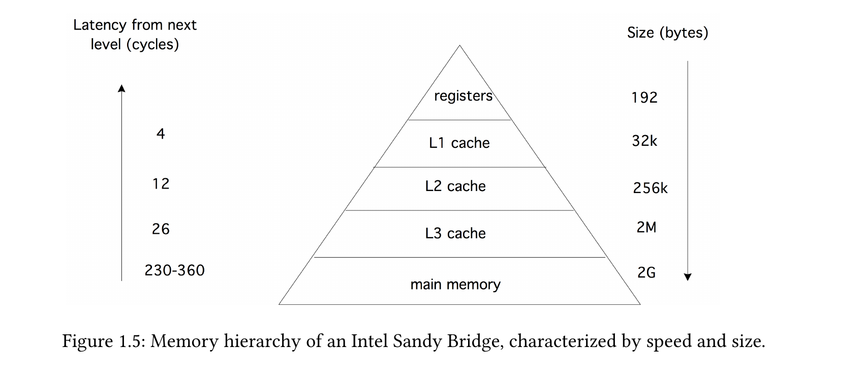
Julia, Fortran, Matlab store column-wise: \(a_{11},a_{21},a_{12},a_{22}\).

This information is important to iterate efficiently over matrices:

function column_major_add(A, B)
    (n,m) = size(A)
    for j = 1:m
        for i = 1:n     # inner loop traverses a column
            A[i,j] += B[i,j]
        end
    end
end

function row_major_add(A, B)
    (n,m) = size(A)
    for i = 1:n
        for j = 1:m     # inner loop traverses a row
            A[i,j] += B[i,j]
        end
    end
end

row_major_add (generic function with 1 method)

A = rand(10000, 10000);
B = rand(10000, 10000);

using BenchmarkTools

@benchmark row_major_add($A, $B)

BenchmarkTools.Trial: 6 samples with 1 evaluation per sample.
 Range (min … max):  905.524 ms … 985.877 ms  ┊ GC (min … max): 0.00% … 0.00%
 Time  (median):     979.043 ms               ┊ GC (median):    0.00%
 Time  (mean ± σ):   956.631 ms ±  39.531 ms  ┊ GC (mean ± σ):  0.00% ± 0.00%

  █                                                     ▁  ▁ ▁▁  
  █▁▁▁▁▁▁▁▁▁▁▁▁▁▁▁▁▁▁▁▁▁▁▁▁▁▁▁▁▁▁▁▁▁▁▁▁▁▁▁▁▁▁▁▁▁▁▁▁▁▁▁▁▁█▁▁█▁██ ▁
  906 ms           Histogram: frequency by time          986 ms <

 Memory estimate: 0 bytes, allocs estimate: 0.

@benchmark column_major_add($A, $B)

BenchmarkTools.Trial: 74 samples with 1 evaluation per sample.
 Range (min … max):  67.467 ms … 76.844 ms  ┊ GC (min … max): 0.00% … 0.00%
 Time  (median):     67.967 ms              ┊ GC (median):    0.00%
 Time  (mean ± σ):   68.172 ms ±  1.087 ms  ┊ GC (mean ± σ):  0.00% ± 0.00%

         ▂  ▁ ▁ █                                              
  ▃▁▁▁▁▁▃█▆▄█▆███▁█▆█▄▃▃▁▁▁▃▁▃▁▃▃▁▁▁▁▁▁▁▃▁▁▁▃▁▄▁▁▁▁▁▁▁▃▁▁▁▁▁▃ ▁
  67.5 ms         Histogram: frequency by time        69.5 ms <

 Memory estimate: 0 bytes, allocs estimate: 0.

12.5.1 Locality of Memory Access and Caching

We have observed that the order of inner and outer loops significantly affects computational efficiency:

It is more efficient when the innermost loop iterates over the left index, i.e., a column rather than a row. This is due to the architecture of modern processors.

Memory access involves multiple cache levels.
A cache miss, which necessitates reloading from slower caches, slows down processing.
To minimize the frequency of cache misses, processors reload larger memory blocks.
Consequently, it is crucial to organize memory access as locally as possible.

Memory hierarchy of Intel processors, from: Victor Eijkhout, *Introduction to High-Performance Scientific Computing*, https://theartofhpc.com/

12.6 Mathematical Operations with Arrays

Arrays of the same dimension (e.g., all \(7\times3\)-matrices) form a linear space.

They can be multiplied by scalars and
they can be added and subtracted.

0.5 * [2, 3, 4, 5]

4-element Vector{Float64}:
 1.0
 1.5
 2.0
 2.5

0.5 * [ 1  3
        2  7] - [ 2  3; 1 2]

2×2 Matrix{Float64}:
 -1.5  -1.5
  0.0   1.5

12.6.1 Matrix Product

The matrix product is defined for

1st factor	2nd factor	Product
\((n\times m)\)-matrix	\((m\times k)\)-matrix	\((n\times k)\)-matrix
\((n\times m)\)-matrix	\(m\)-vector	\(n\)-vector
\((1\times m)\)-row vector	\((m\times n)\)-matrix	\(n\)-vector
\((1\times m)\)-row vector	\(m\)-vector	scalar product
\(m\)-vector	\((1\times n)\)-row vector	\((m\times n)\)-matrix

Examples:

A = [1 2 3
     4 5 6]
v = [2, 3]
w = [1, 3, 4];

(2,3)-matrix * (3,2)-matrix

A * A'

2×2 Matrix{Int64}:
 14  32
 32  77

(3,2)-matrix * (2,3)-matrix

A' * A

3×3 Matrix{Int64}:
 17  22  27
 22  29  36
 27  36  45

(2,3)-matrix * 3-vector

A * w

2-element Vector{Int64}:
 19
 43

(1,2)-vector * (2,3)-matrix

v' * A

1×3 adjoint(::Vector{Int64}) with eltype Int64:
 14  19  24

(3,2)-matrix * 2-vector

A' * v

3-element Vector{Int64}:
 14
 19
 24

(1,2)-vector * 2-vector (scalar product)

v' * v

2-vector * (1,3)-vector (outer product)

v * w'

2×3 Matrix{Int64}:
 2  6   8
 3  9  12

12.7 Broadcasting

With broadcasting, operations or functions are applied element-wise to arrays.
Broadcasting is indicated by a dot preceding an operator or following a function name.
The parser translates f.(x,y) into broadcast(f, x, y), and similarly, x .⊙ y into broadcast(⊙, x, y).
Operands lacking one or more dimensions are virtually replicated in those dimensions.
Broadcasting assignments such as .=, .+=, etc., alter the semantics by modifying values directly within the left-side object (which must have the appropriate dimensions) without creating a new object.
With broadcasting, operations or functions are applied element-wise to arrays.

Some examples:

Element-wise application of a function

sin.([1, 2, 3])

3-element Vector{Float64}:
 0.8414709848078965
 0.9092974268256817
 0.1411200080598672

The following does not give the algebraic square root of a matrix, but the element-wise square root of each entry.

A = [8 2
     3 4]

sqrt.(A)

2×2 Matrix{Float64}:
 2.82843  1.41421
 1.73205  2.0

The following does not give \(A^2\), but the entries are squared.

A.^2

2×2 Matrix{Int64}:
 64   4
  9  16

For comparison, here the results of the algebraic operations:

@show A^2 A^(1/2);

A ^ 2 = [70 24; 36 22]
A ^ (1 / 2) = [2.780234855920959 0.42449510866609885; 0.6367426629991483 1.9312446385887614]

Broadcasting also works with functions of several variables.

hyp(a,b) = sqrt(a^2+b^2)

B = [3 4
     5 7]

hyp.(A, B)

2×2 Matrix{Float64}:
 8.544    4.47214
 5.83095  8.06226

When operands possess differing dimensions, the operand with fewer dimensions is effectively expanded through replication along those dimensions.

Adding a scalar to a matrix:

A = [ 1 2 3
      4 5 6]

2×3 Matrix{Int64}:
 1  2  3
 4  5  6

A .+ 300

2×3 Matrix{Int64}:
 301  302  303
 304  305  306

The scalar was replicated to match the matrix dimensions. Let broadcast() illustrate the form of the second operand after broadcasting:

broadcast( (x,y) -> y, A, 300)

(This replication occurs solely in a virtual sense; the object is not actually instantiated in memory.)

A .+ [10, 20]

2×3 Matrix{Int64}:
 11  12  13
 24  25  26

The vector is expanded by repeating columns:

broadcast((x,y)->y, A, [10,20])

2×3 Matrix{Int64}:
 10  10  10
 20  20  20

Matrix and row vector: The row vector is repeated row-wise:

A .* [1,2,3]'      # adjoint vector

2×3 Matrix{Int64}:
 1   4   9
 4  10  18

The 2nd operand is grown by broadcast() through replication of rows.

broadcast((x,y)->y, A, [1,2,3]')

2×3 Matrix{Int64}:
 1  2  3
 1  2  3

Broadcasting in Assignments

Assignments such as =, +=, /=,… in Julia involve constructing an object on the right-hand side and assigning it to a variable on the left-hand side.

When working with arrays, efficiency often requires reusing existing array objects. The values computed on the right-hand side are then stored directly into the pre-existing object on the left-hand side.

This is accomplished using broadcast variants of assignment operators: .=, .+=,….

A .= 3

2×3 Matrix{Int64}:
 3  3  3
 3  3  3

A .+= [1, 4]

2×3 Matrix{Int64}:
 4  4  4
 7  7  7

12.8 Further Array Functions - a Selection

Julia provides a large number of functions that work with arrays.

A = [22 -17 8 ; 4 6 9]

2×3 Matrix{Int64}:
 22  -17  8
  4    6  9

Find the maximum

maximum(A)

Find the maximum of each column

maximum(A, dims=1)

1×3 Matrix{Int64}:
 22  6  9

Find the maximum of each row

maximum(A, dims=2)

2×1 Matrix{Int64}:
 22
  9

Find the minimum and its position

amin, i = findmin(A)

(-17, CartesianIndex(1, 2))

What is a CartesianIndex?

dump(i)

CartesianIndex{2}
  I: Tuple{Int64, Int64}
    1: Int64 1
    2: Int64 2

Extract the indices of the minimum as a tuple

i.I

(1, 2)

Sum and product of all entries

sum(A), prod(A)

(32, -646272)

Column sum (1st index is reduced)

sum(A, dims=1)

1×3 Matrix{Int64}:
 26  -11  17

Row sums (2nd index is reduced)

sum(A, dims=2)

2×1 Matrix{Int64}:
 13
 19

Sum after applying a function element-wise

sum(x->sqrt(abs(x)), A)   #   sum_ij sqrt(|a_ij|)

19.09143825297046

Reduce (fold) the array with a function

reduce(+, A)    #  equivalent to sum(A)

mapreduce(f, op, array): Apply f to all entries, then reduce with op


mapreduce(x -> x^2, +, A )     # Sum of the squares of all entries

Are there elements in A that are > 5?

any(x -> x>5, A)

true

How many elements in A are > 5?

count(x-> x>5, A)

are all entries positive?

all(x-> x>0, A)

false