6 Machine Numbers

for x ∈ ( 3, 3.3e4,  Int16(20), Float32(3.3e4), UInt16(9) )
    @show x sizeof(x) typeof(x)
    println()
end

x = 3
sizeof(x) = 8
typeof(x) = Int64

x = 33000.0
sizeof(x) = 8
typeof(x) = Float64

x = 20
sizeof(x) = 2
typeof(x) = Int16

x = 33000.0f0
sizeof(x) = 4
typeof(x) = Float32

x = 0x0009
sizeof(x) = 2
typeof(x) = UInt16

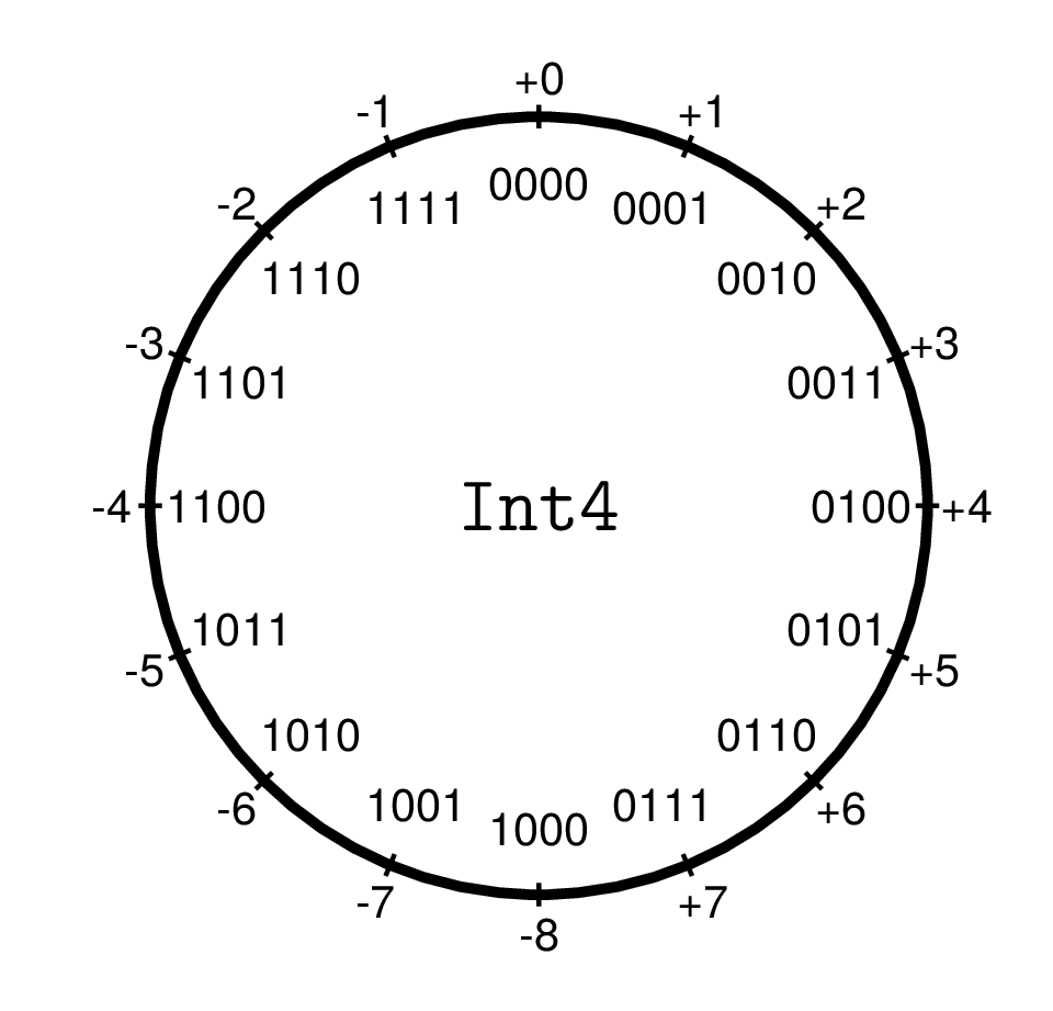
6.1 Integers

Integers are stored as fixed-length bit patterns. Therefore, the value range is finite. Within this value range addition, subtraction, multiplication, and integer division with remainder are exact operations without rounding errors.

Integer numbers come in two types: Signed and Unsigned, which can be viewed as machine models for ℤ and ℕ respectively.

6.1.1 Unsigned integers

subtypes(Unsigned)

5-element Vector{Any}:
 UInt128
 UInt16
 UInt32
 UInt64
 UInt8

UInts are binary numbers with a bit width of 8, 16, 32, 64, or 128 and the corresponding value range of \[ 0 \le x < 2^n \] They are used rarely in scientific computing. In low-level hardware programming, they are used, e.g., for handling binary data and memory addresses. By default, Julia displays them as hexadecimal numbers (with prefix 0x and digits 0-9a-f).

x = 0x0033efef
@show x typeof(x) Int(x)

z = UInt(32)
@show z typeof(z);

x = 0x0033efef
typeof(x) = UInt32
Int(x) = 3403759
z = 0x0000000000000020
typeof(z) = UInt64

6.1.2 Signed Integers

subtypes(Signed)

6-element Vector{Any}:
 BigInt
 Int128
 Int16
 Int32
 Int64
 Int8

Integers have the value range \[ -2^{n-1} \le x < 2^{n-1} \]

In Julia, integer numbers are 64-bit by default:

x = 42
typeof(x)

Int64

Therefore, they have the value range: \[ -9.223.372.036.854.775.808 \le x \le 9.223.372.036.854.775.807 \]

32-bit integers have the value range \[ -2.147.483.648 \le x \le 2.147.483.647 \] By the way, the maximum value \(2^{31}-1\) is a Mersenne prime:

using Primes 
isprime(2^31-1)

true

Negative numbers are represented in two’s complement:

\(x \Rightarrow -x\) corresponds to: flip all bits, then add 1

This looks as follows:

A representation of the fictional data type `Int4`

The most significant bit indicates the sign. However, its “flipping” does not correspond to the operation x → -x.

Important

All integer arithmetic is arithmetic modulo \(2^n\)

x = 2^62 - 10 + 2^62

9223372036854775798

x + 20

-9223372036854775798

No error message, no warning! Fixed-length integers do not lie on a line, but on a circle.

Let’s look at a few integers:

using Printf

for i in (1, 2, 7, -7, 2^50, -1, Int16(7), Int8(7))
    s = bitstring(i)
    t = typeof(i)
    @printf "%20i %-5s ⇒  %s\n" i t s 
end

                   1 Int64 ⇒  0000000000000000000000000000000000000000000000000000000000000001
                   2 Int64 ⇒  0000000000000000000000000000000000000000000000000000000000000010
                   7 Int64 ⇒  0000000000000000000000000000000000000000000000000000000000000111
                  -7 Int64 ⇒  1111111111111111111111111111111111111111111111111111111111111001
    1125899906842624 Int64 ⇒  0000000000000100000000000000000000000000000000000000000000000000
                  -1 Int64 ⇒  1111111111111111111111111111111111111111111111111111111111111111
                   7 Int16 ⇒  0000000000000111
                   7 Int8  ⇒  00000111

Julia has functions that provide type information (introspection):

typemin(Int64), typemax(Int64)

(-9223372036854775808, 9223372036854775807)

typemin(UInt64), typemax(UInt64), BigInt(typemax(UInt64))

(0x0000000000000000, 0xffffffffffffffff, 18446744073709551615)

typemin(Int8), typemax(Int8)

(-128, 127)

6.2 Integer Arithmetic

Addition, Multiplication

The operations +,-,* have the usual exact arithmetic modulo \(2^{64}\).

Powers `a^b`

Powers a^n are computed exactly modulo \(2^{64}\) for natural exponents n.
For negative exponents, the result is a Float.
0^0 is naturally equal to 1.

(-2)^63, 2^64, 3^(-3), 0^0

(-9223372036854775808, 0, 0.03703703703703704, 1)

For natural exponents, exponentiation by squaring is used, so for example x^23 requires only 7 multiplications: \[ x^{23} = \left( \left( (x^2)^2 \cdot x \right)^2 \cdot x \right)^2 \cdot x \]

Division

Division / produces a floating-point number.

x = 40/5

8.0

Integer Division and Remainder

The functions div(a,b), rem(a,b), and divrem(a,b) compute the quotient of integer division, the corresponding remainder, or both as a tuple.
For div(a,b) there is the operator form a ÷ b (input: \div<TAB>), and for rem(a,b) the operator form a % b.
By default, division uses “rounding toward zero”, so the corresponding remainder has the same sign as the dividend a:

@show divrem( 27, 4)
@show ( 27 ÷  4,  27 %  4)   
@show (-27 ÷  4, -27 %  4 )
@show ( 27 ÷ -4,  27 % -4);

divrem(27, 4) = (6, 3)
(27 ÷ 4, 27 % 4) = (6, 3)
(-27 ÷ 4, -27 % 4) = (-6, -3)
(27 ÷ -4, 27 % -4) = (-6, 3)

A rounding rule other than RoundToZero can be specified as the third optional argument for these functions.
?RoundingMode shows the possible rounding modes.
For the rounding rule RoundDown (“toward minus infinity” – so that the corresponding remainder has the same sign as the divisor b), there are also the functions fld(a,b) (floored division) and mod(a,b):

@show divrem(-27, 4, RoundDown)
@show (fld(-27,  4), mod(-27,  4))
@show (fld( 27, -4), mod( 27, -4));

divrem(-27, 4, RoundDown) = (-7, 1)
(fld(-27, 4), mod(-27, 4)) = (-7, 1)
(fld(27, -4), mod(27, -4)) = (-7, -1)

For all rounding modes, the following holds:

div(a, b, RoundingMode) * b + rem(a, b, RoundingMode) = a

The `BigInt` Type

The BigInt type supports arbitrary-precision integers with dynamically allocated memory.

Numeric constants automatically have a sufficiently large type:

z = 10
@show typeof(z)
z = 10_000_000_000_000_000    # 10 quadrillion
@show typeof(z)
z = 10_000_000_000_000_000_000  # 10 quintillion
@show typeof(z)
z = 10_000_000_000_000_000_000_000_000_000_000_000_000_000   # 10 sextillion
@show typeof(z);

typeof(z) = Int64
typeof(z) = Int64
typeof(z) = Int128
typeof(z) = BigInt

In most cases, you must explicitly specify the BigInt type to avoid modulo \(2^{64}\) arithmetic:

@show 3^300        BigInt(3)^300;

3 ^ 300 = 4157753088978724465
BigInt(3) ^ 300 = 136891479058588375991326027382088315966463695625337436471480190078368997177499076593800206155688941388250484440597994042813512732765695774566001

Arbitrary precision arithmetic comes at a cost of significant memory and computation time.

We compare the time and memory requirements for summing 10 million integers as Int64 versus BigInt.

# 10^7 random numbers, uniformly distributed between -10^7 and 10^7 
vec_int = rand(-10^7:10^7, 10^7)

# The same numbers as BigInts
vec_bigint = BigInt.(vec_int)

10000000-element Vector{BigInt}:
  1552342
 -9405309
 -3287697
 -6957172
  7906631
 -2272384
  6674556
 -3076566
   411596
 -3667357
        ⋮
  7860807
  9834428
 -2977646
  3679895
  2271996
  2786825
 -9293127
  6949692
  9397632

The @time macro provides a rough estimate of the required time and memory:

@time x = sum(vec_int)
@show x typeof(x)

  0.002977 seconds (46 allocations: 2.125 KiB)
x = 17784527794
typeof(x) = Int64
Int64

@time x = sum(vec_bigint)
@show x typeof(x);

  0.080422 seconds (18 allocations: 856 bytes)
x = 17784527794
typeof(x) = BigInt

Due to Julia’s just-in-time compilation, timing a single function call is not very informative. The BenchmarkTools package provides the @benchmark macro, which calls a function multiple times and displays the execution times as a histogram.

using BenchmarkTools

@benchmark sum($vec_int)

BenchmarkTools.Trial: 1793 samples with 1 evaluation per sample.
 Range (min … max):  2.621 ms …   8.171 ms  ┊ GC (min … max): 0.00% … 0.00%
 Time  (median):     2.748 ms               ┊ GC (median):    0.00%
 Time  (mean ± σ):   2.783 ms ± 288.289 μs  ┊ GC (mean ± σ):  0.00% ± 0.00%

      ▁▄▆█▆▆▅█▄▃ ▁                                             
  ▃▃▄▇█████████████▇▆▆▄▅▄▄▃▃▃▃▃▃▃▃▂▂▂▁▁▂▂▂▂▂▂▁▁▁▁▁▁▁▁▂▁▁▂▁▁▁▂ ▄
  2.62 ms         Histogram: frequency by time        3.31 ms <

 Memory estimate: 0 bytes, allocs estimate: 0.

@benchmark sum($vec_bigint)

BenchmarkTools.Trial: 69 samples with 1 evaluation per sample.
 Range (min … max):  72.618 ms … 81.348 ms  ┊ GC (min … max): 0.00% … 0.00%
 Time  (median):     73.371 ms              ┊ GC (median):    0.00%
 Time  (mean ± σ):   73.438 ms ±  1.062 ms  ┊ GC (mean ± σ):  0.00% ± 0.00%

  ▁ ▄▄█▄   ▁▁   ▁ ▁█▁ ▁▁▁ ▄▁▁▄   █ ▄▄                          
  █▁████▆▆▁██▁▁▆█▁███▁███▁████▆▆▆█▆██▆▁▆▆▁▆▁▁▁▁▁▁▆▁▁▁▁▁▁▁▁▁▁▆ ▁
  72.6 ms         Histogram: frequency by time        74.6 ms <

 Memory estimate: 72 bytes, allocs estimate: 3.

The BigInt addition is more than 30 times slower.

6.3 Floating-Point Numbers

In numerical mathematics, the term machine numbers is also commonly used.

6.3.1 Basic Idea

A “fixed number of digits before and after the decimal point” is unsuitable for many problems.
A separation between “significant digits” and magnitude (mantissa and exponent), as in scientific notation, is much more flexible. \[ 345.2467 \times 10^3\qquad 34.52467\times 10^4\qquad \underline{3.452467\times 10^5}\qquad 0.3452467\times 10^6\qquad 0.03452467\times 10^7\]
For uniqueness, one must choose one of these forms. In the mathematical analysis of machine numbers, one often chooses the form where the first digit after the decimal point is nonzero. Thus, for the mantissa \(m\): \[ 1 > m \ge (0.1)_b = b^{-1}, \]
where \(b\) denotes the base of the number system.
We choose the form that corresponds to the actual implementation on the computer and specify: The representation with exactly one nonzero digit before the decimal point is the normalized representation. Thus, \[ (10)_b = b> m \ge 1. \]
For binary numbers 1.01101, this digit is always equal to one, and one can omit storing this digit. This actually stored (shortened) mantissa we denote by \(M\), so that \[m = 1 + M\] holds.

Machine Numbers

The set of machine numbers \(𝕄(b, p, e_{min}, e_{max})\) is characterized by the base \(b\), the mantissa length \(p\), and the value range of the exponent \(\{e_{min}, ... ,e_{max}\}\).

In our convention, the mantissa of a normalized machine number has one digit (of base \(b\)) before the decimal point and \(p-1\) digits after the decimal point.

If \(b=2\), one needs only \(p-1\) bits to store the mantissa of normalized floating-point numbers.

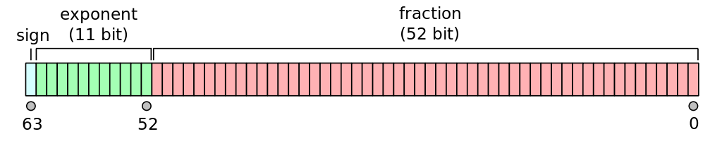
The IEEE 754 standard, implemented by most modern processors and programming languages, defines

Float32 as \(𝕄(2, 24, -126, 127 )\) and
Float64 as \(𝕄(2, 53, -1022, 1023 ).\)

6.3.2 Structure of `Float64` according to the IEEE 754 standard

1 sign bit \(S\)
11 bits for the exponent, thus \(0\le E \le 2047\)
The values \(E=0\) and \(E=(11111111111)_2=2047\) are reserved for encoding special values such as \(\pm0, \pm\infty\), NaN (Not a Number) and subnormal numbers.
52 bits for the (shortened) mantissa \(M,\quad 0\le M<1\), corresponding to approximately 16 decimal digits
Thus, the number represented is: \[ x=(-1)^S \cdot(1+M)\cdot 2^{E-1023}\]

An example:

x = 27.56640625
bitstring(x)

"0100000000111011100100010000000000000000000000000000000000000000"

This can be displayed more clearly:

function printbitsf64(x::Float64)
    s = bitstring(x)
    printstyled(s[1], color = :blue, reverse=true)
    printstyled(s[2:12], color = :green, reverse=true)
    printstyled(s[13:end], color=:red, bold=true, reverse=true)
    print("\n")
end

printbitsf64(x)

0100000000111011100100010000000000000000000000000000000000000000

and we can read S (blue), E (green), and M (red): \[ \begin{aligned} S &= 0\\ E &= (10000000011)_2 = 2^{10} + 2^1 + 2^0 = 1027\\ M &= (.1011100100001)_2 = \frac{1}{2} + \frac{1}{2^3} + \frac{1}{2^4} + \frac{1}{2^5} + \frac{1}{2^8} + \frac{1}{2^{12}}\\ x &=(-1)^S \cdot(1+M)\cdot 2^{E-1023} \end{aligned} \]

… and thus reconstruct the number:

x = (1 + 1/2 + 1/8 + 1/16 + 1/32 + 1/256 + 1/4096) * 2^4

27.56640625

The set of machine numbers 𝕄 forms a finite, discrete subset of ℝ. There exists a smallest and a largest machine number; all other elements x∈𝕄 have both a predecessor and successor in 𝕄.
What is the successor of x in 𝕄? To do this, we set the smallest mantissa bit from 0 to 1.
Converting a string of zeros and ones into the corresponding machine number:

ux = parse(UInt64, "0100000000111011100100010000000000000000000000000000000000000001", base=2)
reinterpret(Float64, ux)

27.566406250000004

However, Julia can do this more simply:

y = nextfloat(x)

27.566406250000004

The predecessor of x is:

z = prevfloat(x)
println(z)
printbitsf64(z)

27.566406249999996
0100000000111011100100001111111111111111111111111111111111111111

6.4 Machine Epsilon

The distance between 1 and its successor nextfloat(1) is called machine epsilon.
For Float64 with a mantissa length of 52 bits, \(\epsilon=2^{-52}\).

@show nextfloat(1.) - 1   2^-52   eps(Float64);

nextfloat(1.0) - 1 = 2.220446049250313e-16
2 ^ -52 = 2.220446049250313e-16
eps(Float64) = 2.220446049250313e-16

Machine epsilon measures the relative distance between machine numbers and quantifies the statement: “64-bit floating-point numbers have a precision of approximately 16 decimal digits.”
Machine epsilon should not be confused with the smallest positive floating-point number:

floatmin(Float64)

2.2250738585072014e-308

Part of the literature uses a different definition of machine epsilon, which is half as large. \[ \epsilon' = \frac{\epsilon}{2}\approx 1.1\times 10^{-16} \] This is the maximum relative error that can occur when rounding a real number to the nearest machine number.
Since numbers in the interval \((1-\epsilon',1+\epsilon']\) are rounded to the machine number \(1\), one can also define \(\epsilon'\) as: the largest number for which \(1+\epsilon' = 1\) still holds in machine arithmetic.

This allows to compute machine epsilon using the floating point arithmetic:

Eps = 1
while(1 != 1 + Eps)
    Eps /= 2
    println(1+Eps)
end
Eps

1.5
1.25
1.125
1.0625
1.03125
1.015625
1.0078125
1.00390625
1.001953125
1.0009765625
1.00048828125
1.000244140625
1.0001220703125
1.00006103515625
1.000030517578125
1.0000152587890625
1.0000076293945312
1.0000038146972656
1.0000019073486328
1.0000009536743164
1.0000004768371582
1.000000238418579
1.0000001192092896
1.0000000596046448
1.0000000298023224
1.0000000149011612
1.0000000074505806
1.0000000037252903
1.0000000018626451
1.0000000009313226
1.0000000004656613
1.0000000002328306
1.0000000001164153
1.0000000000582077
1.0000000000291038
1.000000000014552
1.000000000007276
1.000000000003638
1.000000000001819
1.0000000000009095
1.0000000000004547
1.0000000000002274
1.0000000000001137
1.0000000000000568
1.0000000000000284
1.0000000000000142
1.000000000000007
1.0000000000000036
1.0000000000000018
1.0000000000000009
1.0000000000000004
1.0000000000000002
1.0
1.1102230246251565e-16

or as a bit pattern:

Eps=1
while 1 != 1 + Eps
    Eps/= 2
    printbitsf64(1+Eps)
end
Eps

0011111111111000000000000000000000000000000000000000000000000000
0011111111110100000000000000000000000000000000000000000000000000
0011111111110010000000000000000000000000000000000000000000000000
0011111111110001000000000000000000000000000000000000000000000000
0011111111110000100000000000000000000000000000000000000000000000
0011111111110000010000000000000000000000000000000000000000000000
0011111111110000001000000000000000000000000000000000000000000000
0011111111110000000100000000000000000000000000000000000000000000
0011111111110000000010000000000000000000000000000000000000000000
0011111111110000000001000000000000000000000000000000000000000000
0011111111110000000000100000000000000000000000000000000000000000
0011111111110000000000010000000000000000000000000000000000000000
0011111111110000000000001000000000000000000000000000000000000000
0011111111110000000000000100000000000000000000000000000000000000
0011111111110000000000000010000000000000000000000000000000000000
0011111111110000000000000001000000000000000000000000000000000000
0011111111110000000000000000100000000000000000000000000000000000
0011111111110000000000000000010000000000000000000000000000000000
0011111111110000000000000000001000000000000000000000000000000000
0011111111110000000000000000000100000000000000000000000000000000
0011111111110000000000000000000010000000000000000000000000000000
0011111111110000000000000000000001000000000000000000000000000000
0011111111110000000000000000000000100000000000000000000000000000
0011111111110000000000000000000000010000000000000000000000000000
0011111111110000000000000000000000001000000000000000000000000000
0011111111110000000000000000000000000100000000000000000000000000
0011111111110000000000000000000000000010000000000000000000000000
0011111111110000000000000000000000000001000000000000000000000000
0011111111110000000000000000000000000000100000000000000000000000
0011111111110000000000000000000000000000010000000000000000000000
0011111111110000000000000000000000000000001000000000000000000000
0011111111110000000000000000000000000000000100000000000000000000
0011111111110000000000000000000000000000000010000000000000000000
0011111111110000000000000000000000000000000001000000000000000000
0011111111110000000000000000000000000000000000100000000000000000
0011111111110000000000000000000000000000000000010000000000000000
0011111111110000000000000000000000000000000000001000000000000000
0011111111110000000000000000000000000000000000000100000000000000
0011111111110000000000000000000000000000000000000010000000000000
0011111111110000000000000000000000000000000000000001000000000000
0011111111110000000000000000000000000000000000000000100000000000
0011111111110000000000000000000000000000000000000000010000000000
0011111111110000000000000000000000000000000000000000001000000000
0011111111110000000000000000000000000000000000000000000100000000
0011111111110000000000000000000000000000000000000000000010000000
0011111111110000000000000000000000000000000000000000000001000000
0011111111110000000000000000000000000000000000000000000000100000
0011111111110000000000000000000000000000000000000000000000010000
0011111111110000000000000000000000000000000000000000000000001000
0011111111110000000000000000000000000000000000000000000000000100
0011111111110000000000000000000000000000000000000000000000000010
0011111111110000000000000000000000000000000000000000000000000001
0011111111110000000000000000000000000000000000000000000000000000
1.1102230246251565e-16

The Set of (normalized) Machine Numbers

In the interval \([1,2)\) there are \(2^{52}\) equidistant machine numbers.
After that, the exponent increases by 1 and the mantissa \(M\) is reset to 0. Thus, the interval \([2,4)\) again contains \(2^{52}\) equidistant machine numbers, as does the interval \([4,8)\) up to \([2^{1023}, 2^{1024})\).
Likewise, in the intervals \(\ [\frac{1}{2},1), \ [\frac{1}{4},\frac{1}{2}),...\) there are \(2^{52}\) equidistant machine numbers each, down to \([2^{-1022}, 2^{-1021})\).
This forms the set \(𝕄_+\) of positive machine numbers, and we have \[ 𝕄 = -𝕄_+ \cup \{0\} \cup 𝕄_+ \]

The largest and smallest positive representable normalized floating-point numbers of a floating-point type can be queried:

@show floatmax(Float64)
printbitsf64(floatmax(Float64))

@show floatmin(Float64)
printbitsf64(floatmin(Float64))

floatmax(Float64) = 1.7976931348623157e308
0111111111101111111111111111111111111111111111111111111111111111
floatmin(Float64) = 2.2250738585072014e-308
0000000000010000000000000000000000000000000000000000000000000000

6.5 Rounding to Machine Numbers

The map rd: ℝ \(\rightarrow\) 𝕄 should round to the nearest representable number.
Standard rounding mode is round to nearest, ties to even: when a value falls exactly midway between two machine numbers (tie), the one with 0 as its last mantissa bit is selected.
Justification: this way, we round up in 50% of the cases and down in 50% of the cases, thus avoiding a “statistical drift” in longer calculations.
It holds: \[ \frac{|x-\text{rd}(x)|}{|x|} \le \frac{1}{2} \epsilon \]

6.6 Machine Number Arithmetic

The machine numbers, as a subset of ℝ, are not algebraically closed. Even the sum of two machine numbers is generally not representable as a machine number.

Important

The IEEE 754 standard requires that machine number arithmetic produces the rounded exact result:

The result must be equal to the one that would result from an exact execution of the corresponding operation followed by rounding. \[ a \oplus b = \text{rd}(a + b) \] The same must hold for the implementation of standard functions such as sqrt(), log(), sin(), … – they also return the machine number closest to the exact result.

Arithmetic is not associative:

1 +  10^-16 + 10^-16

1.0

1 + (10^-16 + 10^-16)

1.0000000000000002

In the first case (without parentheses), evaluation proceeds from left to right: \[ \begin{aligned} 1 \oplus 10^{-16} \oplus 10^{-16} &= (1 \oplus 10^{-16}) \oplus 10^{-16} \\ &= \text{rd}\left(\text{rd}(1 + 10^{-16}) + 10^{-16} \right)\\ &= \text{rd}(1 + 10^{-16})\\ &= 1 \end{aligned} \]

In the second case, one obtains: \[ \begin{aligned} 1 \oplus \left(10^{-16} \oplus 10^{-16}\right) &= \text{rd}\left(1 + \text{rd}(10^{-16} + 10^{-16}) \right)\\ &= \text{rd}(1 + 2*10^{-16})\\ &= 1.0000000000000002 \end{aligned} \]

One should also remember that even “simple” decimal fractions cannot always be represented exactly as machine numbers:

\[ \begin{aligned} (0.1)_{10} &= (0.000110011001100110011001100...)_2 = (0.000\overline{1100})_2 \\ (0.3)_{10} &= (0.0100110011001100110011001100..)_2 = (0.0\overline{1001})_2 \end{aligned} \]

printbitsf64(0.1)
printbitsf64(0.3)

0011111110111001100110011001100110011001100110011001100110011010
0011111111010011001100110011001100110011001100110011001100110011

Consequence:

0.1 + 0.1 == 0.2

true

0.2 + 0.1 == 0.3

false

0.2 + 0.1

0.30000000000000004

When outputting a machine number, the binary fraction must be converted to a decimal fraction. Julia can display more digits of this decimal fraction expansion:

using Printf
@printf("%.30f", 0.1)

0.100000000000000005551115123126

@printf("%.30f", 0.3)

0.299999999999999988897769753748

The binary fraction mantissa of a machine number can have a long or even infinitely periodic decimal expansion. But one should not be misled into thinking that this is “higher precision”!

Important

Key message: When testing Floats for equality, one should almost always define a realistic tolerance epsilon appropriate to the problem and test:

epsilon = 1.e-10

if abs(x-y) < epsilon
   # ...
end

6.7 Normalized and Subnormal Machine Numbers

The gap between zero and the smallest normalized machine number \(2^{-1022} \approx 2.22\times 10^{-308}\) is filled with subnormal machine numbers.

Let’s look at a simple model:

Let 𝕄(10,4,±5) be the set of machine numbers to base 10 with 4 mantissa digits (one before the decimal point, 3 after) and the exponent range -5 ≤ E ≤ 5.
Then the normalized representation (nonzero leading digit) of e.g. 1234.0 is 1.234e3 and of 0.00789 is 7.890e-3.
It is essential that machine numbers remain normalized at each computation step. Only then is the full mantissa length utilized, maximizing accuracy.
The smallest positive normalized number in our model is x = 1.000e-5. Already x/2 would have to be rounded to 0.
But for many applications, it is advantageous to allow also subnormal numbers and represent x/2 as 0.500e-5 or x/20 as 0.050e-5.
This gradual underflow is of course associated with a loss of significant digits and thus accuracy.

In the Float data type, such subnormal values are represented by an exponent field in which all bits are equal to zero:

using Printf

x = 2 * floatmin(Float64)   # 2*smallest normalized floating-point number > 0

while x != 0
    x /= 2
    @printf "%14.6g  " x
    printbitsf64(x)
end

  2.22507e-308  0000000000010000000000000000000000000000000000000000000000000000
  1.11254e-308  0000000000001000000000000000000000000000000000000000000000000000
  5.56268e-309  0000000000000100000000000000000000000000000000000000000000000000
  2.78134e-309  0000000000000010000000000000000000000000000000000000000000000000
  1.39067e-309  0000000000000001000000000000000000000000000000000000000000000000
  6.95336e-310  0000000000000000100000000000000000000000000000000000000000000000
  3.47668e-310  0000000000000000010000000000000000000000000000000000000000000000
  1.73834e-310  0000000000000000001000000000000000000000000000000000000000000000
  8.69169e-311  0000000000000000000100000000000000000000000000000000000000000000
  4.34585e-311  0000000000000000000010000000000000000000000000000000000000000000
  2.17292e-311  0000000000000000000001000000000000000000000000000000000000000000
  1.08646e-311  0000000000000000000000100000000000000000000000000000000000000000
  5.43231e-312  0000000000000000000000010000000000000000000000000000000000000000
  2.71615e-312  0000000000000000000000001000000000000000000000000000000000000000
  1.35808e-312  0000000000000000000000000100000000000000000000000000000000000000
  6.79039e-313  0000000000000000000000000010000000000000000000000000000000000000
  3.39519e-313  0000000000000000000000000001000000000000000000000000000000000000
   1.6976e-313  0000000000000000000000000000100000000000000000000000000000000000
  8.48798e-314  0000000000000000000000000000010000000000000000000000000000000000
  4.24399e-314  0000000000000000000000000000001000000000000000000000000000000000
    2.122e-314  0000000000000000000000000000000100000000000000000000000000000000
    1.061e-314  0000000000000000000000000000000010000000000000000000000000000000
  5.30499e-315  0000000000000000000000000000000001000000000000000000000000000000
  2.65249e-315  0000000000000000000000000000000000100000000000000000000000000000
  1.32625e-315  0000000000000000000000000000000000010000000000000000000000000000
  6.63124e-316  0000000000000000000000000000000000001000000000000000000000000000
  3.31562e-316  0000000000000000000000000000000000000100000000000000000000000000
  1.65781e-316  0000000000000000000000000000000000000010000000000000000000000000
  8.28905e-317  0000000000000000000000000000000000000001000000000000000000000000
  4.14452e-317  0000000000000000000000000000000000000000100000000000000000000000
  2.07226e-317  0000000000000000000000000000000000000000010000000000000000000000
  1.03613e-317  0000000000000000000000000000000000000000001000000000000000000000
  5.18065e-318  0000000000000000000000000000000000000000000100000000000000000000
  2.59033e-318  0000000000000000000000000000000000000000000010000000000000000000
  1.29516e-318  0000000000000000000000000000000000000000000001000000000000000000
  6.47582e-319  0000000000000000000000000000000000000000000000100000000000000000
  3.23791e-319  0000000000000000000000000000000000000000000000010000000000000000
  1.61895e-319  0000000000000000000000000000000000000000000000001000000000000000
  8.09477e-320  0000000000000000000000000000000000000000000000000100000000000000
  4.04739e-320  0000000000000000000000000000000000000000000000000010000000000000
  2.02369e-320  0000000000000000000000000000000000000000000000000001000000000000
  1.01185e-320  0000000000000000000000000000000000000000000000000000100000000000
  5.05923e-321  0000000000000000000000000000000000000000000000000000010000000000
  2.52962e-321  0000000000000000000000000000000000000000000000000000001000000000
  1.26481e-321  0000000000000000000000000000000000000000000000000000000100000000
  6.32404e-322  0000000000000000000000000000000000000000000000000000000010000000
  3.16202e-322  0000000000000000000000000000000000000000000000000000000001000000
  1.58101e-322  0000000000000000000000000000000000000000000000000000000000100000
  7.90505e-323  0000000000000000000000000000000000000000000000000000000000010000
  3.95253e-323  0000000000000000000000000000000000000000000000000000000000001000
  1.97626e-323  0000000000000000000000000000000000000000000000000000000000000100
  9.88131e-324  0000000000000000000000000000000000000000000000000000000000000010
  4.94066e-324  0000000000000000000000000000000000000000000000000000000000000001
             0  0000000000000000000000000000000000000000000000000000000000000000

6.8 Special Values

Floating-point arithmetic defines certain special values, e.g.,

nextfloat(floatmax(Float64))

Inf

for x ∈ (NaN, Inf, -Inf, -0.0)
    @printf "%6g  " x
    printbitsf64(x)
end

   NaN  0111111111111000000000000000000000000000000000000000000000000000
   Inf  0111111111110000000000000000000000000000000000000000000000000000
  -Inf  1111111111110000000000000000000000000000000000000000000000000000
    -0  1000000000000000000000000000000000000000000000000000000000000000

An exponent overflow leads to the result Inf or -Inf.

2/0, -3/0, floatmax(Float64) * 1.01, exp(1300)

(Inf, -Inf, Inf, Inf)

One can continue calculating with these values:

-Inf + 20, Inf/30, 23/-Inf, sqrt(Inf),  Inf * 0, Inf - Inf

(-Inf, Inf, -0.0, Inf, NaN, NaN)

NaN (Not a Number) represents the result of an undefined operation. All further operations with NaN also result in NaN.

0/0, Inf - Inf, 2.3NaN, sqrt(NaN)

(NaN, NaN, NaN, NaN)

Since NaN represents an undefined value, it is not equal to anything, not even to itself. This is sensible, because if two variables x and y are computed as NaN, one should not conclude that they are equal.
There is therefore a boolean function isnan() to test for NaN.

x = 0/0
y = Inf - Inf
@show x==y   NaN==NaN  isfinite(NaN) isinf(NaN) isnan(x) isnan(y);

x == y = false
NaN == NaN = false
isfinite(NaN) = false
isinf(NaN) = false
isnan(x) = true
isnan(y) = true

There is a “minus zero”. It signals a numerical underflow of a small negative quantity.

@show 23/-Inf   -2/exp(1200)    -0.0==0.0;

23 / -Inf = -0.0
-2 / exp(1200) = -0.0
-0.0 == 0.0 = true

6.9 Mathematical Functions

Julia has the usual mathematical functions
sqrt, exp, log, log2, log10, sin, cos,..., asin, acos,..., sinh,..., gcd, lcm, factorial,...,abs, max, min,...,

including e.g. the rounding functions

floor(T,x) = \(\lfloor x \rfloor\)
ceil(T,x) = \(\lceil x \rceil\)

floor(3.4),   floor(Int64, 3.5),   floor(Int64, -3.5)

(3.0, 3, -4)

ceil(3.4),    ceil(Int64, 3.5),    ceil(Int64, -3.5)

(4.0, 4, -3)

Also worth noting is atan(y, x), the two-argument arctangent (known as atan2 in many programming languages, see atan2). This solves the problem of converting from Cartesian to polar coordinates without awkward case distinctions.

atan(y,x) is the angle of the polar coordinates of (x,y) in the interval \((-\pi,\pi]\). In the 1st and 4th quadrants, it is therefore equal to atan(y/x)

atan(3, -2),    atan(-3, 2),    atan(-3/2)

(2.1587989303424644, -0.982793723247329, -0.982793723247329)

6.10 Conversion Between Strings and Numbers

Use the functions parse() and string() for such conversions:

parse(Int64, "1101", base=2)

string(13, base=2)

"1101"

string(1/7)

"0.14285714285714285"

string(77, base=16)

"4d"

For conversion of numerical types into each other, one can use the type names. Type names are also constructors:

x = Int8(67)
@show x   typeof(x);

x = 67
typeof(x) = Int8

z = UInt64(3459)

0x0000000000000d83

y = Float64(z)

3459.0

6.11 Literature

D. Goldberg, What Every Computer Scientist Should Know About Floating-Point Arithmetic
C. Vuik, Some Disasters caused by numerical errors

Source: Codekaizen, CC BY-SA 4.0, via Wikimedia Commons ↩︎

6.1 Integers

6.1.1 Unsigned integers

6.1.2 Signed Integers

6.2 Integer Arithmetic

Addition, Multiplication

Powers a^b

Division

Integer Division and Remainder

The BigInt Type

6.3 Floating-Point Numbers

6.3.1 Basic Idea

6.3.2 Structure of Float64 according to the IEEE 754 standard

6.4 Machine Epsilon

6.5 Rounding to Machine Numbers

6.6 Machine Number Arithmetic

6.7 Normalized and Subnormal Machine Numbers

6.8 Special Values

6.9 Mathematical Functions

6.10 Conversion Between Strings and Numbers

6.11 Literature

Powers `a^b`

The `BigInt` Type

6.3.2 Structure of `Float64` according to the IEEE 754 standard